Plot reaction time distributions

Visualize reaction time distributions from your model predictions. Overlay observed experimental data for reference.

Usage

plot_rt(simulated_output, observed_df, facet_x = c("item_idx"), facet_y = c())

Arguments

simulated_output

Output from run_simulation containing posterior predictions

observed_df

Your observed data as a data frame

facet_x

Variables to split plots horizontally. Default is "item_idx" to show separate plots for each item

facet_y

Variables to split plots vertically. Default is none (c())

Value

A plot showing predicted RT distributions (blue), with observed data (red) if provided

Details

Posterior predictions are first summarized to their median RT within each condition and facet group before plotting. This provides a representative estimate from the posterior distribution rather than pooling all individual trial-level predictions.

Examples

# Load example posterior simulation output
post_output_path <- system.file(
  "extdata", "rdm_minimal", "abc", "posterior", "neuralnet",
  package = "eam"
)
post_output <- load_simulation_output(post_output_path)

# Load example observed data
obs_file <- system.file(
  "extdata", "rdm_minimal", "observation", "observation_data.csv",
  package = "eam"
)
obs_df <- read.csv(obs_file)

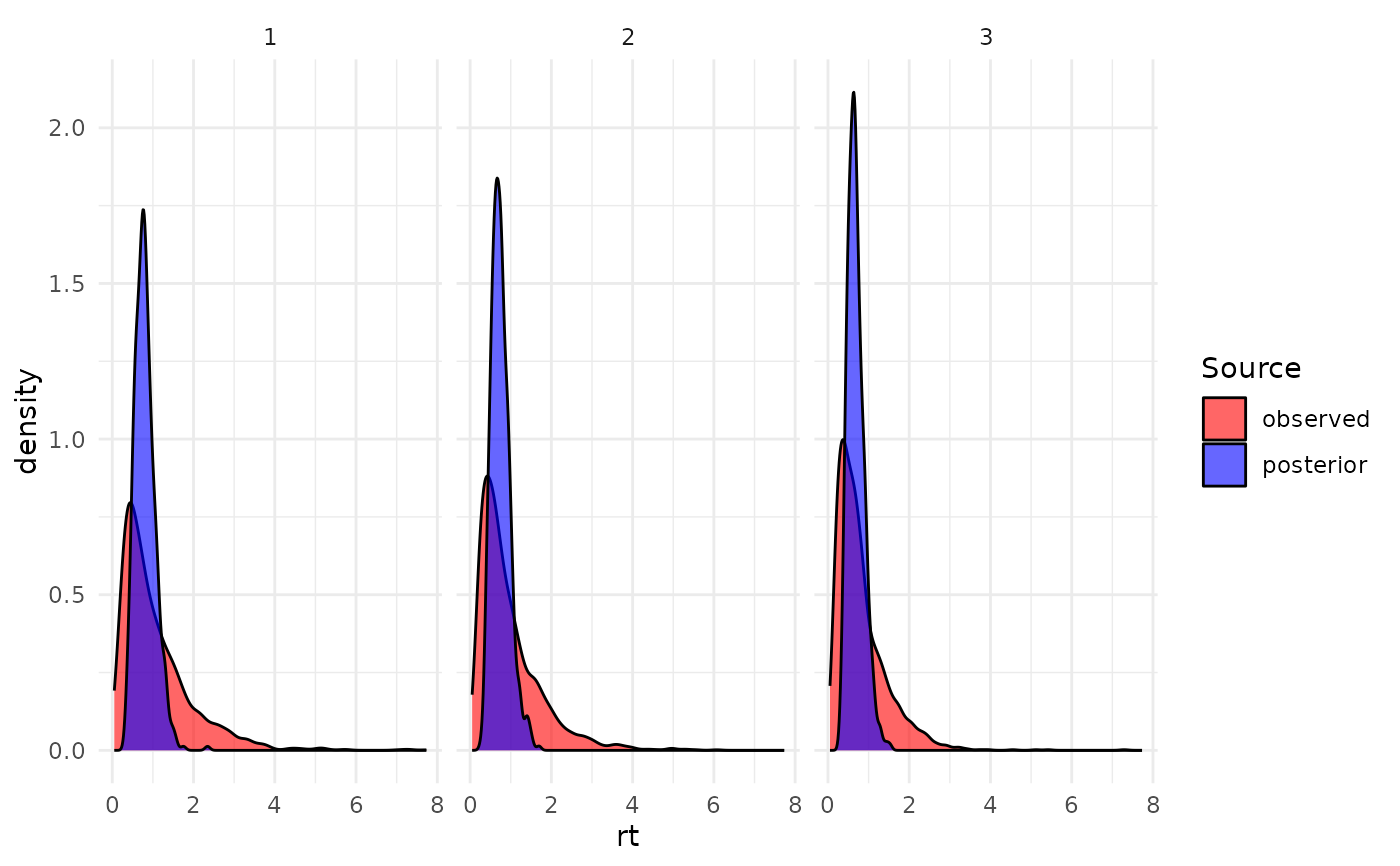
# Plot RT distributions by item
plot_rt(post_output, obs_df, facet_x = c("item_idx"))


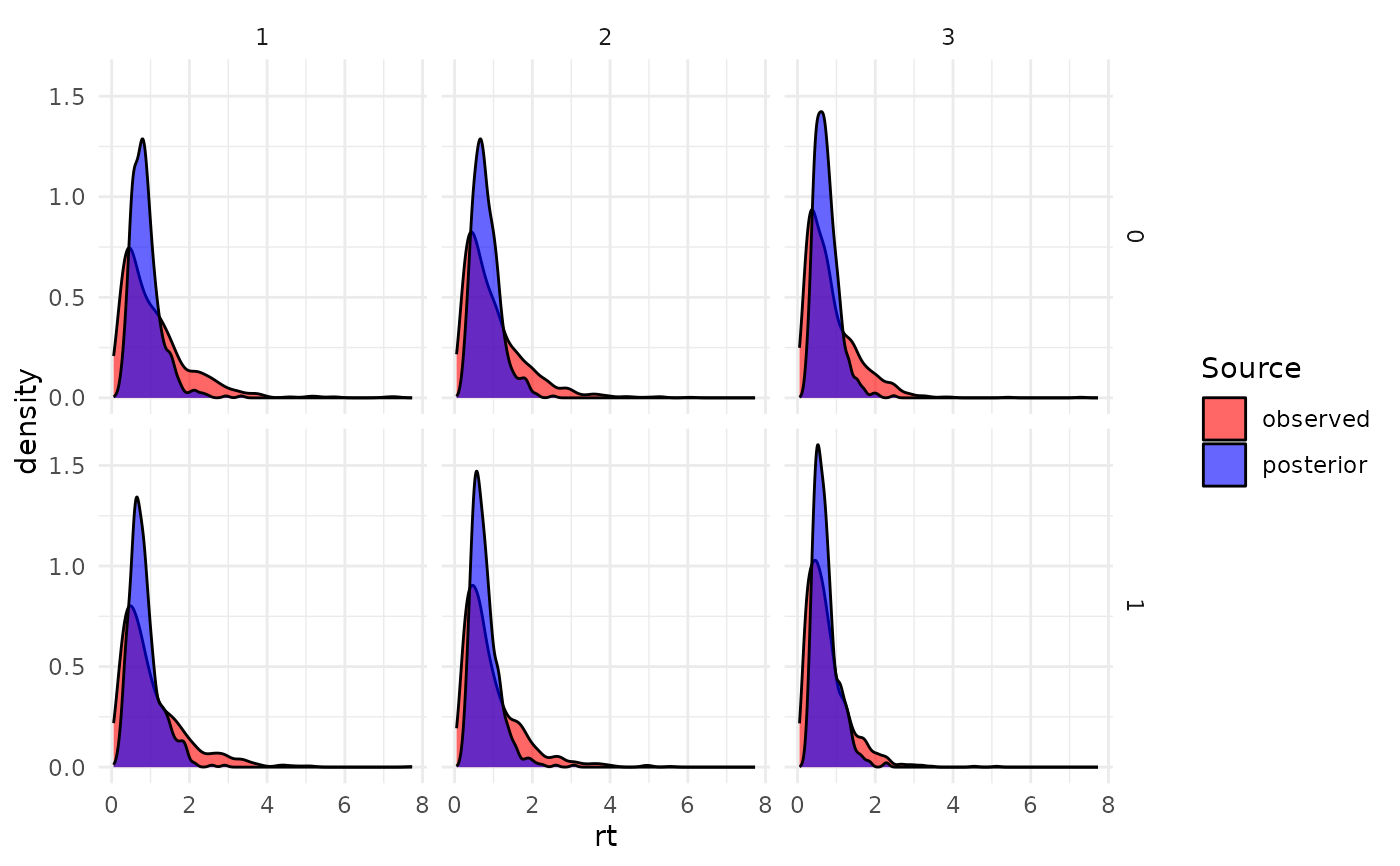
# Plot RT distributions by item and group
plot_rt(
  post_output,
  obs_df,
  facet_x = c("item_idx"),
  facet_y = c("group")
)